Defining Variables

You can define information about your variables by accessing the Variable View tab (at the bottom of the Data Editor window). The Variable View tab displays information about the variables in your data. You can get to the Variable View window in two ways:

• In the Data Editor window, click the Variable View tab at the bottom.
• In the Data Editor window, in the Data View tab, double-click a variable name at the top of the column. This method has the advantage of taking you to the specific variable you clicked.

The Variable View tab displays the following information, in columns, about each variable in your data:

NAME

The name of the variable, which is used to refer to that variable in syntax. Variable names can not contain spaces. Note that when you change the name of a variable, it does not change the data; all values associated with the variable stay the same. Renaming a variable simply changes the name of that variable while leaving everything else the same. For example, we may want to rename a variable called Sex to Gender.

To change a variable’s name, double-click on the name of the variable that you wish to re-name. Type your new variable name.

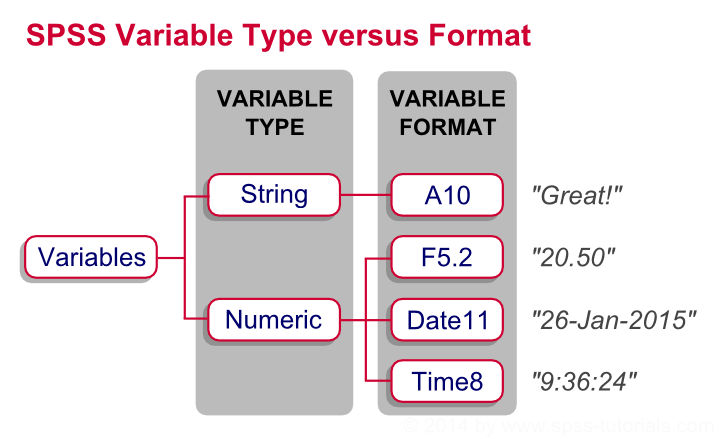
TYPE

The type of variable (e.g. numeric, string, etc.). (See the Variable Types tutorial for descriptions of the variable types in SPSS.)

To change a variable’s type, click inside the cell corresponding to the “Type” column for that variable. A square “…” button will appear; click on it to open the Variable Type window. Click the option that best matches the type of variable. Click OK.

WIDTH

The number of digits displayed for numerical values or the length of a string variable.

To set a variable’s width, click inside the cell corresponding to the “Width” column for that variable. Then click the “up” or “down” arrow icons to increase or decrease the number width.

DECIMALS

The number of digits to display after a decimal point for values of that variable. Does not apply to string variables. Note that this changes how the numbers are displayed, but does not change the values in the dataset.

To specify the number of decimal places for a numeric variable, click inside the cell corresponding to the “Decimals” column for that variable. Then click the “up” or “down” arrow icons to increase or decrease the number of decimal places.

Example: If you specify that values should have two decimal points, they will display as 1.00, 2.00, 3.00, and so on.

LABEL

A brief but descriptive definition or display name for the variable. When defined, a variable’s label will appear in the output in place of its name.

Example: The variable expgradate might be described by the label “Expected date of college graduation”.

VALUES

For coded categorical variables, the value label(s) that should be associated with each category abbreviation. Value labels are useful primarily for categorical (i.e., nominal or ordinal) variables, especially if they have been recorded as codes (e.g., 1, 2, 3). It is strongly suggested that you give each value a label so that you (and anyone looking at your data or results) understands what each value represents.

When value labels are defined, the labels will display in the output instead of the original codes.Note that defining value labels only affects the labels associated with each value, and does not change the recorded values themselves.

Example: In the sample dataset, the variable Rank represents the student’s class rank. The values 1, 2, 3, 4 represent the categories Freshman, Sophomore, Junior, and Senior, respectively. Let’s define the category labels for the Rank variable in the sample data.

Under the column “Values,” click the cell that corresponds to the variable whose values you wish to label. If the values are currently undefined, the cell will say “None.” Click the square “…” button. The Value Labels window appears.

Type the first possible value (1) for your variable in the Value field. In the Label field type the label exactly as you want it to display (e.g., “Freshman”). Click Add when you are finished defining the value and label. Your variable value and label will appear in the center box. Repeat these steps for each possible value for your variable. When all of the labels have been defined, the Value Labels window should look like this:

Click OK at the bottom of the window.

If you wish to change or remove a value and label that you have added to the center dialog box, do the following:

• To change a specific value or label, highlight the value/label in the center text box in the Value Labels window. Now the selected value/label will be highlighted yellow. Make changes to the selected value or label as needed. Click Change. The changes will be applied to the value/label you highlighted.
• To remove a specific value/label, highlight the value/label in the center text box. Click Remove. The selected value/label will be removed from the center text box.

MISSING

The user-defined values that indicate data are missing for a variable (e.g., -99). Note that this does not affect or eliminate SPSS’s default missing value code (“.”). This column merely allows the user to specify alternative codes for missing values.

To set user-defined missing value codes, click inside the cell corresponding to the “Missing” column for that variable. A square button will appear; click on it.

The Missing Values window appears.

Click the option that best matches how you wish to define missing data and enter any associated values, then click OK at the bottom of the window.

COLUMNS

The width of each column in the Data View spreadsheet. Note that this is not the same as the number of digits displayed for each value. This simply refers to the width of the actual column in the spreadsheet.

To set a variable’s column width, click inside the cell corresponding to the “Columns” column for that variable. Then click the “up” or “down” arrow icons to increase or decrease the column width.

ALIGN

The alignment of content in the cells of the SPSS Data View spreadsheet. Options include left-justified, right-justified, or center-justified.

To set the alignment for a variable, click inside the cell corresponding to the “Align” column for that variable. Then use the drop-down menu to select your preferred alignment: Left, Right, or Center.

MEASURE

The level of measurement for the variable (e.g., nominal, ordinal, or scale).

Some procedures in SPSS treat categorical and scale variables differently. By default, variables with numeric responses are automatically detected as “Scale” variables. If the numeric responses actually represent categories, you must change the specified measurement level to the appropriate setting.

To define a variable’s measurement level, click inside the cell corresponding to the “Measure” column for that variable. Then click the drop-down arrow to select the level of measurement for that variable: Scale, Ordinal, or Nominal.

It is vital that you correctly define each variable’s measurement level. This setting affects everything from graphs to internal algorithms for statistical analysis. Incorrectly specifying measurement level can have unintended and potentially disastrous effects on your results.

ROLE

The role that a variable will play in your analyses (i.e., independent variable, dependent variable, both independent and dependent). Some options in SPSS allow you to pre-select variables for particular analyses based on their defined roles. Any variable that meets the role requirements will be available for use in such analyses. You can choose from the following roles for each variable:

• Input: The variable will be used as a predictor (independent variable). This is the default assignment for variables.
• Target: The variable will be used as an outcome (dependent variable).
• Both: The variable will be used as both a predictor and an outcome (independent and dependent variable).
• None: The variable has no role assignment.
• Partition: The variable will partition the data into separate samples.
• Split: Used with the IBM® SPSS® Modeler (not IBM® SPSS® Statistics).

To define a variable’s role in your analysis, click inside the cell corresponding to the “Role” column for that variable. Then use the drop-down menu to select the role that variable will take: Input, Target, Both, None, Partition, or Split.

VARIABLE NAMES

CHANGE AN EXISTING VARIABLE’S NAME

Rename one variable:

RENAME VARIABLES (oldname=newname). 

Rename more than one variable:

RENAME VARIABLES (oldname=newname) (oldname2=newname2) (oldname3=newname3). 

VARIABLE WIDTH

Set the width for one variable:

VARIABLE WIDTH var1 (10).

Set the same width for multiple variables:

VARIABLE WIDTH var1 var2 var3 (10).

Set different widths for multiple variables:

VARIABLE WIDTH var1 var2 var3 (10)
/ var4 var5 (20)
/ var6 (5).

VARIABLE MEASUREMENT LEVEL

Set the measurement level (nominal, ordinal, or scale) for one or more variables at a time:

VARIABLE LEVEL var1 var2 var3 (SCALE).

VARIABLE LEVEL var4 var5 (ORDINAL).

VARIABLE LEVEL var6 (NOMINAL).

Set more than one variable’s measurement level at a time:

VARIABLE LEVEL var1 var2 var3 (SCALE)
/ var4 var5 (ORDINAL).
/ var6 (NOMINAL).

VARIABLE LABELS

Set label for one variable:

VARIABLE LABELS varname "Variable label".

Set labels for several variables:

VARIABLE LABELS var1 "Variable 1 label" var2 "Variable 2 label" var3 "Variable 3 label".

VALUE LABELS

Define labels for one numeric variable’s values:

VALUE LABELS var1 0 'No' 1 'Yes'.

Define labels for one string variable’s values:

VALUE LABELS var2 'm' 'Male' 'f' 'Female'.

Define the same set of labels for more than one numeric variable (e.g. you have several 5-point Likert items that all use the same coding scheme):

VALUE LABELS service quality speed overall 
-2 'Very unsatisfied' 
-1 'Somewhat unsatisfied' 
1 'Somewhat satisfied' 
2 'Very satisfied'.

VALUE LABELS likert1 TO likert10 
1 'Strongly disagree' 
2 'Disagree' 
3 'Neither agree nor disagree' 
4 'Agree' 
5 'Strongly agree'.

Define more than one set of labels at a time:

VALUE LABELS married smoker 0 'No' 1 'Yes'
  / sex 1 'Male' 2 'Female'.

MISSING VALUE CODES

Define one special missing value for a single numeric variable:

MISSING VALUES num1 (-999).

Define more than one special missing value for a single numeric variable:

MISSING VALUES num1 (-999, -888).

Define a set of missing value codes to be applied to several numeric variables:

MISSING VALUES num1 num2 num3 (-999, -888).

Define one special missing value for a single string variable:

MISSING VALUES string1 ('x').

Define more than one special missing value for a single string variable:

MISSING VALUES string1 ('x', 'missing', '-999').

Define different sets of special missing values for different variables:

MISSING VALUES num1 num2 (-99, -88) string1 ('x', 'missing') string2 ('-999').

Reset missing value codes for all variables:

MISSING VALUES ALL ().

The Define Variable Properties window is an efficient way of defining many variables at once, or defining many variables that share the same formatting. Click Data > Define Variable Properties.

The Define Variable Properties window will open.

The left column displays all of the variables in your dataset. Select the variables you wish to define and move them to the right column using the arrow button. Note that you can specify the number of cases to scan, as well as the number of values that will display in the next step. Click Continue when you have finished selecting variables.

A second window will appear; this one allows you to define various properties for each variable you selected.

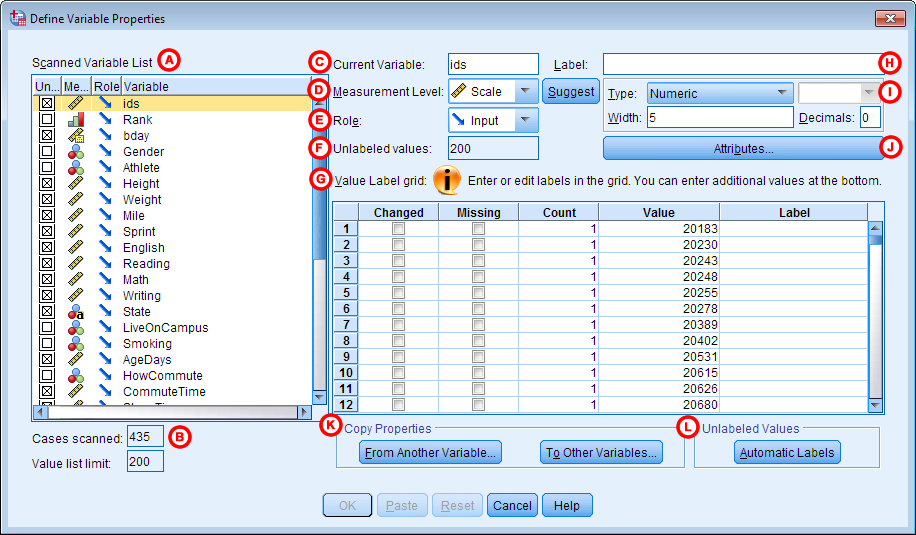
A Scanned Variable List: The “Scanned Variable List” column includes the variables selected in the previous step. Variables that do not have assigned value labels will have an X in the “Unlabeled” column. For example, if the variable Gender has potential values of “1” and “2” but these values are not labeled (e.g., “male” and “female”, respectively), the Unlabeled values check box will be selected for this variable. The current Measurement Level and Role for each variable is also displayed.

B  Cases scanned: This section displays the number of cases that were scanned for each selected variable, as well as the number of values that are listed in the Value Label grid (G).

C Current Variable: Displays the variable that is currently selected from the Scanned Variable List (A).

D Measurement Level: Displays the level of measurement for the selected variable. You can change the level of measurement by clicking the menu arrow and choosing the desired measurement level from the listed options: Scale, Ordinal, Nominal. You can also see the suggested level of measurement for your selected variable. To do this, click Suggest; this will open a new window that will display the currently selected variable, the current measurement level, and SPSS’s suggested level of measurement. SPSS also provides an explanation for the suggestion, and a description of each possible type of measurement level (nominal, ordinal, scale) to help you make a decision.

E Role: Displays the role for the selected variable. Some options in SPSS allow you to pre-select variables for particular analyses based on their defined roles. Any variable that meets the role requirements will be available for use in such analyses. You can change the role by clicking the menu arrow and choosing the desired role from the listed options: Input, Target, Both, None, Partition, Split.

F Unlabeled Values: Specifies how many values do not have corresponding value labels.

G Value Label grid: Displays current information about the selected variable and updates the information based on any changes you make.

Label: Displays value labels that have already been specified for the variable. You can change value labels by clicking on cells beneath the “Label” column and typing labels for each value specified in the “Value” column. If there are values you wish to label that are not currently displayed, you can enter the values in the “Value” column below the last value listed.

Value: The values for the selected variable. Note: The values are based on the specified number of scanned cases (B).

Count: The number of times a value occurs. Note: The count is based on the specified number of scanned cases (B).

Missing: Defines values as missing data. To mark certain values as missing data, simply check the box under “Missing” for the associated value under the “Value” column. Note: If a variable already has defined missing values (e.g., -99), you cannot change the missing values using the Define Variables Properties window. Instead, you will need to go to Variable View and specify any changes in the “Missing” column.

Changed: If you change the value label of a variable, the row associated with the changed value label will automatically be check-marked under the “Changed” column.

H Label: Allows you to add a label for the selected variable that describes more about what the variable is. This label is for the variable rather than for the values of the variable. For example, we might select the variable StudentID and give it the label “Student ID #”.

I Type: Allows you to specify a particular kind of variable that helps SPSS know how to work with the variable during analyses. The types include numeric, comma, dot, scientific, date, dollar currency percent, string, and restricted numeric. Depending on the type you select for your variable, you may be asked to supply additional information. For example, if you select “Date” as the type, you will then be able to select the format of the date from a drop-down menu to the right. You can also set the width and may be asked to set the decimals for your variable. Notice that when you select a particular type for the variable, examples of how the variable would display in your data appear in the Value Label grid area under “Value.”

J Attributes: Allows you to define custom attributes for variables. These attributes are supplementary information not otherwise specified by the variable’s label, measurement labels, and missing values.

K Copy Properties: Allows you to copy properties from one variable to another variable. You can copy the properties from another variable to the currently selected variable, or copy the properties of the currently selected variable to one or more other variables. (For example, you may have several variables representing survey items, all of which use the value labels 0 = “No” and 1 = “Yes”. After defining the value labels for the first item, you can use “Copy Properties” to quickly set the labels for the remaining survey item variables.)

L Unlabeled Values: Allows you to automatically label unlabeled values by clicking Automatic Labels.

When you are finished defining your variables, click OK at the bottom of the window to apply the changes to your data.

As we mentioned at the beginning of this tutorial, it is important to define the variables in your data so that you (and anyone else working with your data) can easily understand what was measured, and how. In this section, we provide an example of the confusion that can result when value labels are not defined, and how to correct it.

In the sample data, the variable Gender has two possible values: 0 and 1. The sample data file is not formatted with any value labels. Let’s make a Frequency table of the Gender variable to see what the distribution of gender is in our sample. Click Analyze > Descriptive Statistics > Frequencies. Select the variable Gender, then click OK. (The Frequencies command will produce a frequency table.) The Output Viewer displays the following results:

This output shows frequencies for the variable Gender, which can take on values of “0” or “1.” We see that value “0” has 204 cases and value “1” has 222 cases. But what do these values mean? Which values represent females, and which values represent males? There is no commonly accepted coding scheme for gender, so readers not familiar with the data can not be certain what is represented in this table.

In the sample data, 0 represents a Male, and 1 represents a Female. After defining the value labels (using the methods described above) and re-running the Frequencies command, the output is much easier for the reader to understand:

It may also be useful to rewrite the labels so that the numeric code is included with the label. In this situation, we could alter the label for “male” to “Male (0)”, and alter the label for “female” to “Female (1)”.

As you can see from this example, including value labels for each variable makes working with data and interpreting output much more straightforward. And remember: value labels are only one of many attributes that we can define for each variable. The more information you define about each variable, the easier it will be to navigate your data and interpret the output of analyses.

Suppose you have conducted a survey that has a time limit, and want to be able to distinguish respondents who refused to answer a question from respondents who ran out of time.

Respondents who refused to answer a survey item are coded as -99. Respondents who did not complete the survey item in the alotted time are coded as -77. All other missing responses were left blank.

To have SPSS recognize these special missing value codes, you’ll need to these numbersas indicators of missing values under the Variable View tab. Click on the cell corresponding to the “Missing” column for the variable of interest to open the Missing Values window. Click Discrete missing values, then enter the two missing value codes.

TIPS

• You can specify up to three different missing value codes.
• You can apply value labels to missing value codes just like you would to valid categories. This is actually a good practice to use, because the names of missing value codes appear in the output.