
- What is Analysis of Variance?
- Types of Analysis of Variance
- Conceptual Background
- Assumptions for ANOVA
- ANOVA vs T-test
- Two-Way Analysis of Variance (Two-Way ANOVA)
What is Analysis of Variance (ANOVA)?
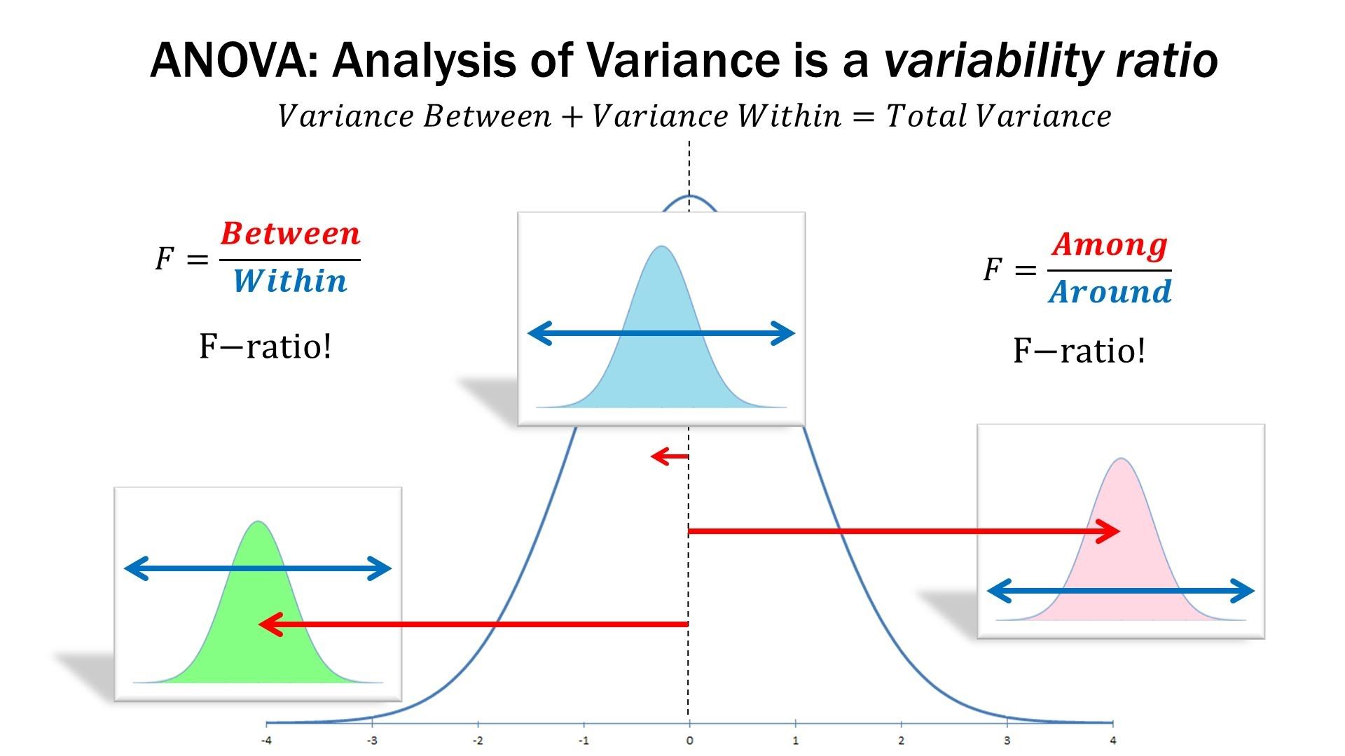
In some decision-making situations, the sample data may be divided into various groups i.e. the sample may be supposed to have consisted of k-sub samples. There are interest lies in examining whether the total sample can be considered as homogenous or there is some indication that sub-samples have been drawn from different populations. So, in these situations, we have to compare the mean values of various groups, with respect to one or more criteria. The total variation present in a set of data may be partitioned into a number of non-overlapping components as per the nature of the classification. The systematic procedure to achieve this is called Analysis of Variance (ANOVA). With the help of such a partitioning, some testing of hypothesis may be performed.
Initially, Analysis of Variance (ANOVA) had been employed only for the experimental data from the Randomized Designs but later they have been used for analyzing survey and secondary data from the Descriptive Research.
Analysis of Variance may also be visualized as a technique to examine a dependence relationship where the response (dependence) variable is metric (measured on interval or ratio scale) and the factors (independent variables) are categorical in nature with a number of categories more than two.
Example of ANOVA
Ventura is an FMCG company, selling a range of products. Its outlets have been spread over the entire state. For administrative and planning purpose, Ventura has sub-divided the state into four geographical-regions (Northern, Eastern, Western and Southern). Random sample data of sales collected from different outlets spread over the four geographical regions.
Variation, being a fundamental characteristics of data, would always be present. Here, the total variation in the sales may be measured by the squared sum of deviation from the mean sales. If we analyze the sources of variation in the sales, in this case, we may identify two sources:
- Sales within a region would differ and this would be true for all four regions (within-group variations)
- There might be impact of the regions and mean-sales of the four regions would not be all the same i.e. there might be variation among regions (between-group variations).
So, total variation present in the sample data may be partitioned into two components: between-regions and within-regions and their magnitudes may be compared to decide whether there is a substantial difference in the sales with respect to regions. If the two variations are in close agreement, then there is no reason to believe that sales are not same in all four regions and if not then it may be concluded that there exists a substantial difference between some or all the regions.
Here, it should be kept in mind that ANOVA is the partitioning of variation as per the assignable causes and random component and by this partitioning ANOVA technique may be used as a method for testing significance of difference among means (more than two).
Types of Analysis of Variance (ANOVA)
If the values of the response variable have been affected by only one factor (different categories of single factor), then there will be only one assignable reason by which data is sub-divided, then the corresponding analysis will be known as One-Way Analysis of Variance. The example (Ventura Sales) comes in this category. Other examples may be: examining the difference in analytical-aptitude among students of various subject-streams (like engineering graduates, management graduates, statistics graduates); impact of different modes of advertisements on brand-acceptance of consumer durables etc.
On the other hand, if we consider the effect of more than one assignable cause (different categories of multiple factors) on the response variable then the corresponding analysis is known as N-Way ANOVA (N>=2). In particular, if the impact of two factors (having multiple categories) been considered on the dependent (response) variable then that is known as Two-Way ANOVA. For example: in the Ventura Sales, if along with geographical-regions (Northern, Eastern, Western and Southern), one more factor ‘type of outlet’ (Rural and Urban) has been considered then the corresponding analysis will be Two-Way ANOVA. More examples: examining the difference in analytical-aptitude among students of various subject-streams and geographical locations; the impact of different modes of advertisements and occupations on brand-acceptance of consumer durables etc.
Two-Way ANOVA may be further classified into two categories:
- Two-Way ANOVA with one observation per cell: there will be only one observation in each cell (combination). Suppose, we have two factors A (having m categories) and B (having n categories), So, there will be N= m*n total observations with one observation(data-point) in each of (Ai Bj) cell (combination), i=1, 2, ……., m and j= 1, 2, …..n. Here, the effect of the two factors may be examined.
- Two-Way ANOVA with multiple observations per cell: there will be multiple observations in each cell (combination). Here, along with the effect of two factors, their interaction effect may also be examined. Interaction effect occurs when the impact of one factor (assignable cause) depends on the category of other assignable cause (factor) and so on. For examining interaction-effect it is necessary that each cell (combination) should have more than one observations so it may not be possible in the earlier Two-Way ANOVA with one observation per cell.
Conceptual Background
The fundamental concept behind the Analysis of Variance is “Linear Model”.
X1, X2,……….Xn are observable quantities. Here, all the values can be expressed as:
Xi = µi + ei
Where µi is the true value which is because of some assignable causes and ei is the error term which is because of random causes. Here, it has been assumed that all error terms ei are independent distributed normal variate with mean zero and common variance (σe2).
Further, true value µi can be assumed to be consist of a linear function of t1, t2,…….tk, known as “effects”.
If in a linear model, all effects tj’s are unknown constants (parameters), then that linear model is known as “fixed-effect model”. Otherwise, if effects tj’s are random variables then that model is known as “random-effect model”.
One-Way Analysis of Variance
We have n observations (Xij), divided into k groups, A1, A2,…….Ak, with each group having nj observations.
Here, the proposed fixed-effect linear model is:
Xij = µi + eij
Where µi is the mean of the ith group.
General effect (grand mean): µ = Σ (ni. µi)/n
and additional effect of the ith group over the general effect: αi = µi – µ.
So, the linear model becomes:
Xij = µ + αi + eij
with Σi (ni αi) = 0
The least-square estimates of µ and αi may be determined by minimizing error sum of square (Σi Σj eij2) = Σi Σj (Xij – µ – αi)2 as:
X.. (combined mean of the sample) and Xi. (mean of the ith group in the sample).
So, the estimated linear model becomes:
Xij = X.. + (Xi.- X..) + (Xij– Xi.)
This can be further solved as:
Σi Σj (Xij –X..)2 = Σi ni (Xi.- X..)2 + Σi Σj (Xij –Xi.)2
Total Sum of Square = Sum of square due to group-effect + Sum of square due to error
or
Total Sum of Square= Between Group Sum of square+ Within Group Sum of square
TSS= SSB + SSE
Further, Mean Sum of Square may be given as:
MSB = SSB/(k-1) and MSE = SSE/(n-k),
where (k-1) is the degree of freedom (df) for SSB and (n-k) is the df for SSE.
Here, it should be noted that SSB and SSE added up to TSS and the corresponding df’s (k-1) and (n-k) add up to total df (n-1) but MSB and MSE will not be added up to Total MS.
This by partitioning TSS and total df into two components, we may be able to test the hypothesis:
H0: µ1 = µ2=……….= µk
H1: Not all µ’s are same i.e. at least one µ is different from others.
or alternatively:
H0: α1 = α2=……….= αk =0
H1: Not all α’s are zero i.e. at least one α is different from zero.
MSE has always been an unbiased estimate of σe2 and if H0 is true then MSB will also be an unbiased estimate of σe2.
Further MSB/ σe2 will follow Chi-square (χ2) distribution with(k-1) df and MSE/ σe2 will follow Chi-square (χ2) distribution with(n-k) df. These two χ2 distributions are independent so the ratio of two Chi-square (χ2) variate F= MSB/MSE will follow variance-ratio distribution (F distribution) with (k-1), (n-k) df.
Here, the test-statistic F is a right-tailed test (one-tailed Test). Accordingly, p-value may be estimated to decide about reject/not able to reject of the null hypothesis H0.
If is H0 rejected i.e. all µ’s are not same then rejecting the null hypothesis does not inform which group-means are different from others, So, Post-Hoc Analysis is to be performed to identify which group-means are significantly different from others. Post Hoc Test is in the form of multiple comparison by testing equality of two group-means (two at a time) i.e. H0: µp = µq by using two-group independent samples test or by comparing the difference between sample means (two at a time) with the least significance difference (LSD)/critical difference (CD)
= terror-df*MSE/ (1/np+1/nq )1/2
If observed difference between two means is greater than the LSD/CD then the corresponding Null hypothesis is rejected at alpha level of significance.
Assumptions for ANOVA
Though it has been discussed in the conceptual part just to reiterate it should be ensured that the following assumptions must be fulfilled:
1. The populations from where samples have been drawn should follow a normal distribution.
2. The samples have been selected randomly and independently.
3. Each group should have common variance i.e. should be homoscedastic i.e. the variability in the dependent variable values within different groups is equal.
It should be noted that the Linear Model used in ANOVA is not affected by minor deviations in the assumptions especially if the sample is large.
The Normality Assumption may be checked using Tests of Normality: Shapiro-Wilk Test and Kolmogorov-Smirnov Test with Lilliefors Significance Correction. Here, Normal Probability Plots (P-P Plots and Q-Q Plots) may also be used for checking normality assumption. The assumption of Equality of Variances (homoscedasticity) may be checked using different Tests of Homogeneity of Variances (Levene Test, Bartlett’s test, Brown–Forsythe test etc.).
ANOVA vs T-test
We employ two-independent sample T-test to examine whether there exists a significant difference in the means of two categories i.e. the two samples have come from the same or different populations. The extension to it may be applied to perform multiple T-tests (by taking two at a time) to examine the significance of the difference in the means of k-samples in place of ANOVA. If this is attempted, then the errors involved in the testing of hypothesis (type I and type II error) can’t be estimated correctly and the value of type I error will be much more than alpha (significance level). So, in this situation, ANOVA is always preferred over multiple intendent samples T-tests.
Like, in our example we have four categories of the regions Northern (N), Eastern (E), Western (W) and Southern (S). If we want to compare the population means by using two-independent sample T-test i.e. by taking two categories (groups) at a time. We have to make 4C2 = 6 number of comparisons i.e. six independent samples tests have to performed (Tests comparing N with S, N with E, N with W, E with W, E with S and W with S), Suppose we are using 5% level of significance for the null hypothesis based on six individual T-tests, then type I error will be = 1- (0.95)6 =1-0.735= 0.265 i.e. 26.5%.
One-Way ANOVA in SPSS
- Analyze => Compare Means=> One-Way ANOVA to open relevant dialogue box.

- Dependent variable in the Dependent List box and independent variable in the Factor box are to be entered.

- Press Options… command-button to open One-Way ANOVA: Options sub-dialogue box. Check Descriptive and Homogeneity-of-variance boxes under Statistics. Press Continue to return to the main dialogue box.

- Press Post Hoc… command-button to open One-Way ANOVA: Post Hoc Multiple Comparisons sub-dialogue box. We will get a number of options for multiple comparison tests. We will select an appropriate test and check that (eg. Tukey HSD). Press Continue to return to the main dialogue box.

- Press Ok to have the output.
Here, we consider the example of Ventura Sales, where the sample has been sub-divided into four geographical regions (Northern, Eastern, Western and Southern), so we have four groups. So, the Hypotheses:
Null Hypothesis H0: µN = µE = µW = µS
Alternative Hypothesis H1: Not all µ’s are same i.e. at least one µ is different from others.
| ANOVA | |||||
| Sale of the outlet (Rs.’000) | |||||
| Sum of Squares | df | Mean Square | F | Sig. | |
| Between Groups | 1182.803 | 3 | 394.268 | 10.771 | .000 |
| Within Groups | 2049.780 | 56 | 36.603 | ||
| Total | 3232.583 | 59 |
As per the ANOVA table, Total Sum of Square (TSS)= 3232.583 has been partitioned into two sums of squares: Between Groups Sum of Square (BSS)= 1182.803 and Within Groups Sum of Square (SSE)= 2049.780. The corresponding Mean Sum of Squares are MSB = 394.268 and MSE= 36.603. It is evident that magnitude of the between-group variation is much higher as compared to within-group variation i.e. two variations are not in close agreement then there is reason to believe that sales are not same in all four regions. Further, the Variance Ratio: F statistic = MSB/MSE = 394.268/36.603 = 10.771 appears to be significantly higher than 1 this supports the view that sales are not the same in all four regions. Finally, the p-value (Sig. = 0.000 < 0.05), which is a substantially low value, indicates that the Null Hypothesis H0 may be rejected at 5% level of significance i.e. there exists a substantial difference in the mean sales among some or all the regions.
| Test of Homogeneity of Variances | |||
| Sale of the outlet (Rs.’000) | |||
| Levene Statistic | df1 | df2 | Sig. |
| 1.909 | 3 | 56 | .139 |
The Test of Homogeneity of Variance Table indicates that the assumption of homogeneity of variance (homoscedasticity) has not been violated as the Levene’s Statistics is not significant (p value = 0.139 >0.05) at 5% level of significance.
Post Hoc Tests
Multiple Comparison
Dependent Variable: Sale of the outlet (Rs.’000)
Tukey HSD
| (I) Location of the outlet in the region | (J) Location of the outlet in the region | Mean Difference (I-J) | Std. Error | Sig. |
| Northern | Eastern | 8.636* | 2.850 | .044 |
| Western | 9.897* | 2.621 | .014 | |
| Southern | 16.836* | 2.886 | .000 | |
| Eastern | Northern | -8.636* | 2.850 | .044 |
| Western | 1.261 | 1.738 | .979 | |
| Southern | 8.200* | 2.116 | .012 | |
| Western | Northern | -9.897* | 2.621 | .014 |
| Eastern | -1.261 | 1.738 | .979 | |
| Southern | 6.939* | 1.795 | .033 | |
| Southern | Northern | -16.836* | 2.886 | .000 |
| Eastern | -8.200* | 2.116 | .012 | |
| Western | -6.939* | 1.795 | .033 | |
| *The mean difference is significant at the 0.05 level. |
Finally, Post Hoc Tests have been performed since the null hypothesis H0 has been rejected so we are interested to examine which regions are different. Here, just for the demonstration purpose, Tukey HSD Test have been employed. The test consists of multiple comparisons by testing equality of group-means (two at a time) i.e. H0: µp = µq for each of six pairs.
There is significant difference in the pairs: Northern # Eastern (Sig. = 0.044), Northern # Western (Sig. = 0.014), Northern # Southern (Sig. = 0.000), Eastern # Southern (Sig. = 0.012) and Western # Southern (Sig. = 0.000) but Eastern and Western regions are not significantly different (Sig. = 0.979) with respect to mean-sales. So, it can be proposed that Northern region mean-sales is significantly different from other regions the same is with Southern region mean-sales. Whereas, there is insignificant difference in the mean-sales of Eastern and Western regions but they are significantly different from the Northern and Southern regions.
Two-Way Analysis of Variance (Two-Way ANOVA)
Here, the value of the dependent variable (response variable) may be impacted by two assignable causes (factors). For example: in the Ventura Sales along with geographical regions (Northern, Eastern, Western and Southern), termed as Factor “A”, we want to examine the impact of the type of outlet (Rural and Urban), termed as Factor “B”, on the mean-sales of the outlets.
Here, the proposed fixed-effect Linear Model is:
Xijk = µij + eijk
Where, µij is the true-value of the (i, j)th cell and eijk is the error term. Error term is assumed to be independently normally distributed with zero mean and common variance. µij is further decomposed as:
µij = µ + αi + βj + γij
So, the fixed effect Linear Model becomes:
Xijk = µ + αi + βj + γij+ eijk
Where,
µ = Overall Mean Value
αi = Effect of the Factor Ai
βj = Effect of the Factor Bj
γij = Interaction-Effect of the Factor (AiBj)
eijk = Error Term
The Least-square estimates may be determined by minimizing error sum of square (Σi Σj Σk eijk)2.
Accordingly, the Analysis of Variance is based on the following relation:
Σi Σj Σk (Xijk –X…)2 = np Σi (Xi.. – X…)2 + mp Σj (X.j. –X…)2+ p Σi Σj (Xij. – Xi.. – X.j. +X…)2+ Σi Σj Σk (Xijk – Xij.)2
Total SS = SS due to Factor A + SS due to Factor B + SS due to Interaction of A & B + SS due to Error.
or
TSS = SSA+ SSB+ SS (AB)+ SSE
By partitioning the variation into the above components, we are able to test following hypotheses:
H01: α1 = α2=……….= αm =0 (No Effect of Factor A)
H02: β1 = β2=……….= βn =0 (No Effect of Factor B)
H03: γij =0 for all i and j (Interaction-Effect is absent)
Accordingly, the Mean Sum of Squares given by:
MSA = SSA/(m-1)
MSB = SSB/(n-1)
MS(AB) = SS(AB)/(m-1)(n-1)
MSE = SSE/mn(p-1)
and the Variance Ratios:
FA= MSA/MSE ~ F distribution with (m-1), mn(p-1) df
FB =MSB/MSE ~ F distribution with (n-1), mn(p-1) df
FAB = MS (AB)/MSE ~ F distribution with (m-1)(n-1), mn(p-1) df.
Accordingly, p-values may be estimated to decide about reject/not able to reject the three null hypotheses H01, H02 and H03 respectively.
For more tutorials on data science and analysis concepts, follow our Data Science page. Great Learning also offers comprehensive courses on Data Science and Analytics and Data Science and Business Analytics which prepares you for all kinds of data science roles.
Contributed by: Mr. MH Siddiqui
LinkedIn profile: https://www.linkedin.com/in/masood-siddiqui-7118a71b/